Point-Based Approximate Ambient Occlusion and Color Bleeding
November 2005 (Revised December 2006)
![]()
Point-Based Approximate Ambient Occlusion and Color BleedingNovember 2005 (Revised December 2006) |
|
The purpose of this application note is to provide recipes and examples for computing point-based approximate ambient occlusion and color bleeding using Pixar's RenderMan (PRMan).
The basic idea is to first bake a point cloud containing areas (and optionally color), one point for each micropolygon, to create a point-based representation of the geometry in the scene. Each point is considered a disk that can cause occlusion and/or color bleeding. For efficiency, the algorithm groups distant points (disks) into clusters that are treated as one entity. The computation method is rather similar to efficient n-body simulations in astrophysics and clustering approaches in finite-element global illumination (radiosity). Some of the implementation details also resemble the subsurface scattering method used in PRMan's ptfilter program.
The advantages of our point-based approach are:
The disadvantages are:
    Attribute "cull" "hidden" 0   # don't cull hidden surfaces
    Attribute "cull" "backfacing" 0   # don't cull backfacing surfaces
    Attribute "dice" "rasterorient" 0   # view-independent dicing
This will ensure that all surfaces are represented in the point cloud
file. Add the following display channel definition:
DisplayChannel "float _area"
And assign this shader to all geometry:
Surface "bake_areas" "filename" "foo_area.ptc" "displaychannels" "_area"
The shader is very simple and looks like this:
    surface
    bake_areas( uniform string filename = "", displaychannels = "" )
    {
      normal Nn = normalize(N);
      float a = area(P, "dicing"); // micropolygon area
      float opacity = 0.333333 * (Os[0] + Os[1] + Os[2]); // average opacity

      a *= opacity; // reduce area if non-opaque

      if (a > 0)
        bake3d(filename, displaychannels, P, Nn, "interpolate", 1, "_area", a);

      Ci = Cs * Os;
      Oi = Os;
    }
Rendering even complex scenes with this simple shader should take less than a minute. The number of baked points can be adjusted by changing the image resolution and/or the shading rate. It is often sufficient (for good quality in the next step) to render with shading rate 4 or higher. This shader reduces the area of points on semi-transparent surfaces so that they cause less occlusion. (If this behavior is not desired, just comment out the line in which the area is reduced by the opacity.) The opacity could of course come from texture map lookups — instead of being uniform over each surface as in this shader.
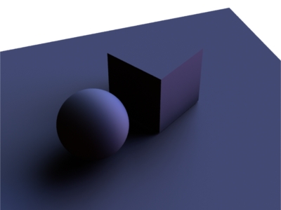
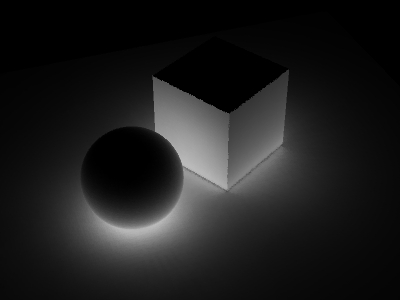
As an example, consider the following rib file:
    FrameBegin 1
      Format 400 300 1
      PixelSamples 4 4
      ShadingRate 4
      ShadingInterpolation "smooth"
      Display "simple_a.tif" "it" "rgba"
      DisplayChannel "float _area"

      Projection "perspective" "fov" 22
      Translate 0 -0.5 8
      Rotate -40  1 0 0
      Rotate -20  0 1 0

      WorldBegin

        Attribute "cull" "hidden" 0   # don't cull hidden surfaces
        Attribute "cull" "backfacing" 0   # don't cull backfacing surfaces
        Attribute "dice" "rasterorient" 0   # view-independent dicing

        Surface "bake_areas" "filename" "simple_areas.ptc"
          "displaychannels" "_area"

        # Ground plane
        AttributeBegin
          Scale 3 3 3
          Polygon "P" [ -1 0 1  1 0 1  1 0 -1  -1 0 -1 ]
        AttributeEnd

        # Sphere
        AttributeBegin
          Translate -0.7 0.5 0
          Sphere 0.5  -0.5 0.5  360
        AttributeEnd

        # Box (with normals facing out)
        AttributeBegin
          Translate 0.3 0.02 0
          Rotate -30  0 1 0
          Polygon "P" [ 0 0 0  0 0 1  0 1 1  0 1 0 ]   # left side
          Polygon "P" [ 1 1 0  1 1 1  1 0 1  1 0 0 ]   # right side
          Polygon "P" [ 0 1 0  1 1 0  1 0 0  0 0 0 ]   # front side
          Polygon "P" [ 0 0 1  1 0 1  1 1 1  0 1 1 ]   # back side
          Polygon "P" [ 0 1 1  1 1 1  1 1 0  0 1 0 ]   # top
          Polygon "P" [ 0 0 0  1 0 0  1 0 1  0 0 1 ]   # bottom
        AttributeEnd
      WorldEnd
    FrameEnd
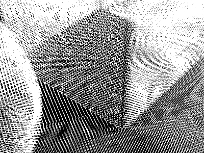
Rendering this scene generates a completely uninteresting image but also a point cloud file called 'simple_areas.ptc'. Displaying the point cloud file using the ptviewer program gives the following image:
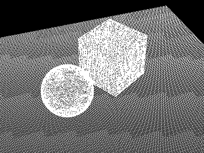 |
(Since the areas are tiny, ptviewer will show a black image by default; just select "Color -> White" to see the points.)
    #include "normals.h"

    surface
    pointbasedocclusion (string filename = "";
	   	         string hitsides = "front";
                         float maxdist = 1e15, falloff = 0, falloffmode = 0,
                         samplebase = 0,
		         clampocclusion = 0, maxsolidangle = 0.05; )
    {
      normal Ns = shadingnormal(N);
      float occ;

      occ = occlusion(P, Ns, 0, "pointbased", 1, "filename", filename,
                      "hitsides", hitsides,
                      "maxdist", maxdist, "falloff", falloff,
                      "falloffmode", falloffmode,
                      "samplebase", samplebase, "clamp", clampocclusion,
                      "maxsolidangle", maxsolidangle);

      Ci = (1 - occ) * Os;
      Oi = Os;
    }
The parameters "hitsides", "maxdist", "falloff", "falloffmode", "samplebase", and "bias" have the same meaning as for the standard, ray-traced ambient occlusion computation. (Note, however, that using "falloff" 0 with a short "maxdist" gives aliased results. We hope to overcome this limitation in a future release.) There will always be a quadratic falloff due to distance; the "falloff" parameter only specifies additional falloff.
The "samplebase" parameter is a number between 0 and 1 and determines jittering of the computation points. A value of 0 (the default) means no jittering, a value of 1 means jittering over the size of a micropolygon. Setting "samplebase" to 0.5 or even 1 can be necessary to avoid thin lines of too low occlusion where two (perpendular) surfaces intersect.
The "bias" parameter offsets the computation points a bit above the original surface. This can be necessary to avoid self-occlusion on highly curved surfaces. Typical values for "bias" will be in the range 0 to 0.001.
The point-based occlusion algorithm will tend to compute too much occlusion. The "clamp" parameter determines whether the algorithm should try to reduce the over-occlusion. Turning on "clamp" roughly doubles the computation time but gives better results.
The "maxsolidangle" parameter is a straightforward time-vs-quality knob. It determines how small a cluster must be (as seen from the point we're computing occlusion for at that time) for it to be a reasonable stand-in for all the points in it. Reasonable values seem to be in the range 0.03 - 0.1.
Implementation detail: The first time the occlusion() function is executed (with the pointbased parameter set to 1) for a given point cloud file it reads in the point cloud file and creates an octree. Each octree node has a spherical harmonic representation of the directional variation of the occlusion caused by the points in that node.
Rib file:
    FrameBegin 1
      Format 400 300 1
      PixelSamples 4 4
      ShadingInterpolation "smooth"
      Display "simple_b.tif" "tiff" "rgba"

      Projection "perspective" "fov" 22
      Translate 0 -0.5 8
      Rotate -40  1 0 0
      Rotate -20  0 1 0

      WorldBegin

        Surface "pointbasedocclusion" "filename" "simple_areas.ptc"

        # Ground plane
        AttributeBegin
          Scale 3 3 3
          Polygon "P" [ -1 0 1  1 0 1  1 0 -1  -1 0 -1 ]
        AttributeEnd

        # Sphere
        AttributeBegin
          Translate -0.7 0.5 0
          Sphere 0.5  -0.5 0.5  360
        AttributeEnd

        # Box (with normals facing out)
        AttributeBegin
          Translate 0.3 0.02 0
          Rotate -30  0 1 0
          Polygon "P" [ 0 0 0  0 0 1  0 1 1  0 1 0 ]   # left side
          Polygon "P" [ 1 1 0  1 1 1  1 0 1  1 0 0 ]   # right side
          Polygon "P" [ 0 1 0  1 1 0  1 0 0  0 0 0 ]   # front side
          Polygon "P" [ 0 0 1  1 0 1  1 1 1  0 1 1 ]   # back side
          Polygon "P" [ 0 1 1  1 1 1  1 1 0  0 1 0 ]   # top
          Polygon "P" [ 0 0 0  1 0 0  1 0 1  0 0 1 ]   # bottom
        AttributeEnd
      WorldEnd
    FrameEnd
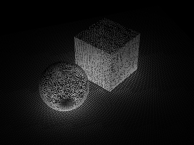
Running this rib file results in the following image:
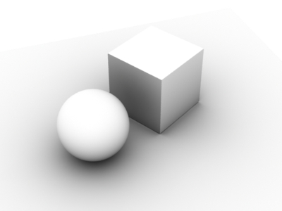 |
The point-based ambient occlusion computation is typically 5-8 times faster than ambient occlusion using ray tracing — at least for complex scenes. (If the scene consists only of a few undisplaced spheres and large polygons, as in this example, ray tracing is faster since ray tracing those geometric primitives does not require fine tessellation.)
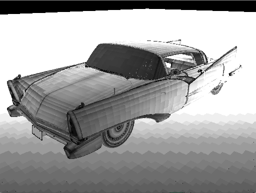
Here is an example of point-based ambient occlusion in a more complex scene:
 |
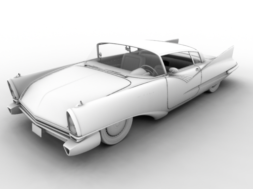 |
Generating the area point cloud takes about two minutes on a standard PC, and computing (and rendering) the point-based ambient occlusion takes less than six minutes.
Keep in mind that the point-based ambient occlusion values are (by their very nature) not exactly the same as the ambient occlusion computed by ray tracing. However, the point-based occlusion has much of the same "look". It is often necessary to try different combinations of "hitsides", "maxdist", "falloff", "falloffmode", "clamp", and "maxsolidangle" to get an occlusion result that closely resembles ray-traced ambient occlusion.
Another issue that can require some fine-tuning can occur where two surfaces intersect. Sometimes a thin line with too little occlusion can be visible along the intersection. To avoid this, set the "samplebase" parameter to 0.5 or 1, and experiment with different values for the "bias" parameter. This issue is similar to ray-tracing bias for ray-traced occlusion.
The environment direction (the average unoccluded direction, also known as "bent normal") can also be computed by the occlusion() function with the point-based approach. Just pass the occlusion() function an "environmentdir" variable, and it will be filled in — just as for ray-traced occlusion() calls. The environment directions will be computed more accurately if the "clamp" parameter is set than if it isn't.
Environment illumination, as for example from an HDRI environment map, can be computed efficiently as a by-product of the point-based occlusion computation.
For an example, replace the surface shader in the example above with:
    #include "normals.h"

    surface
    pointbasedenvcolor (string filename = "";
	    	        string hitsides = "both";
                        float maxdist = 1e15, falloff = 0, falloffmode = 0;
                        float samplebase = 0, bias = 0;
                        float clampocclusion = 1;
                        float maxsolidangle = 0.05;
                        string envmap = "" )
    {
        normal Ns = shadingnormal(N);
        color envcol = 0;
        vector envdir = 0;
        float occ;

        occ = occlusion(P, Ns, 0, "pointbased", 1, "filename", filename,
                        "hitsides", hitsides,
                        "maxdist", maxdist, "falloff", falloff,
		        "falloffmode", falloffmode,
                        "samplebase", samplebase, "bias", bias,
                        "clamp", clampocclusion,
                        "maxsolidangle", maxsolidangle,
		        "environmentmap", envmap,
                        "environmentcolor", envcol,
                        "environmentdir", envdir
                       );

        Ci = envcol;
        Oi = Os;
    }
Change the surface shader call in the rib file to:
    Surface "pointbasedenvcolor" "filename" "simple_areas.ptc"
      "envmap" "rosette_hdr.tex"
The resulting image looks like this:
 |
Here's another example of environment illumination, this time the scene is slightly more complex and the environment map consists of two very bright area lights, one green and one blue:
 |
    surface
    bake_radiosity(string bakefile = "", displaychannels = "", texfile = "";
                    float Ka = 1, Kd = 1)
    {
      color irrad, tex = 1, diffcolor;
      normal Nn = normalize(N);
      float a = area(P, "dicing"); // micropolygon area

      // Compute direct illumination (ambient and diffuse)
      irrad = Ka*ambient() + Kd*diffuse(Nn);

      // Lookup diffuse texture (if any)
      if (texfile != "")
        tex = texture(texfile);

      diffcolor = Cs * tex;

      // Compute Ci and Oi
      Ci = irrad * diffcolor * Os;
      Oi = Os;

      // Store area and Ci in point cloud file
      bake3d(bakefile, displaychannels, P, Nn, "interpolate", 1,
             "_area", a, "_radiosity", Ci, "Cs", diffcolor);
    }
(Here we also bake out the diffuse surface color. That color isn't used in this example, but can be be used to compute multiple bounces of color bleeding using ptfilter; this is discussed in Section 5.)
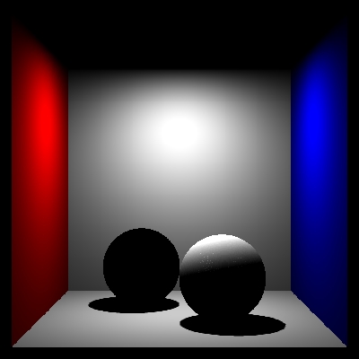
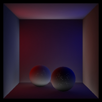
Here is a rib file showing an example. This scene is the infamous Cornell box with two spheres.
    FrameBegin 1
      Format 400 400 1
      ShadingInterpolation "smooth"
      PixelSamples 4 4
      Display "cornell_a.tif" "it" "rgba"
      Projection "perspective" "fov" 30
      Translate 0 0 5

      DisplayChannel "float _area"
      DisplayChannel "color _radiosity"
      DisplayChannel "color Cs"

      WorldBegin

        Attribute "cull" "hidden" 0   # to ensure occl. is comp. behind objects
        Attribute "cull" "backfacing" 0 # to ensure occl. is comp. on backsides
        Attribute "dice" "rasterorient" 0   # view-independent dicing

        LightSource "cosinelight_rts" 1 "from" [0 1.0001 0] "intensity" 4

        Surface "bake_radiosity" "bakefile" "cornell_radio.ptc"
          "displaychannels" "_area,_radiosity,Cs" "Kd" 0.8

        # Matte box
        AttributeBegin
          Color [1 0 0]
          Polygon "P" [ -1 1 -1  -1 1 1  -1 -1 1  -1 -1 -1 ]   # left wall
          Color [0 0 1]
          Polygon "P" [ 1 -1 -1  1 -1 1  1 1 1  1 1 -1 ]   # right wall
          Color [1 1 1]
          Polygon "P" [ -1 1 1  1 1 1  1 -1 1  -1 -1 1 ]   # back wall
          Polygon "P" [ -1 1 -1  1 1 -1  1 1 1  -1 1 1 ]   # ceiling
          Polygon "P" [ -1 -1 1  1 -1 1  1 -1 -1  -1 -1 -1 ]   # floor
        AttributeEnd

        Attribute "visibility" "transmission" "opaque" # the spheres cast shadows

        # Left sphere (chrome; set to black in this pass)
        AttributeBegin
          color [0 0 0]
          Translate -0.3 -0.69 0.3
          Sphere 0.3  -0.3 0.3  360
        AttributeEnd

        # Right sphere (matte)
        AttributeBegin
          Translate 0.3 -0.69 -0.3
          Sphere 0.3  -0.3 0.3  360
        AttributeEnd
      WorldEnd
    FrameEnd
Running this rib file results in the following image:
 |
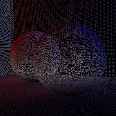
The generated point cloud, cornell_radio.ptc, contains approximately 545,000 points. The figure below shows two views of it (with the radiosity color shown):
 |
 |
Now we are ready to compute and render point-based color bleeding using the indirectdiffuse() function. This can be done using a shader similar to this example:
    #include "normals.h"

    surface
    pointbasedcolorbleeding (string filename = "", sides = "front";
	   	   	     float clampbleeding = 1, sortbleeding = 1,
                             maxdist = 1e15, falloff = 0, falloffmode = 0,
                             samplebase = 0, bias = 0,
                             maxsolidangle = 0.05;)
    {
      normal Ns = shadingnormal(N);
      color irr = 0;
      float occ = 0;

      irr = indirectdiffuse(P, Ns, 0, "pointbased", 1, "filename", filename,
                            "hitsides", sides,
                            "clamp", clampbleeding,
                            "sortbleeding", sortbleeding,
                            "maxdist", maxdist, "falloff", falloff,
                            "falloffmode", falloffmode,
                            "samplebase", samplebase, "bias", bias,
                            "maxsolidangle", maxsolidangle);

      Ci = Os * Cs * irr;
      Oi = Os;
    }
New for PRMan 13.0.4: The indirectdiffuse() function has a new parameter called 'sortbleeding'. Clamp must be 1 for it to have any effect. When sortbleeding is 1, the bleeding colors are sorted according to distance and composited correctly, i.e. nearby points block light from more distant points. This gives more correct colors and deeper (darker) shadows. When sortbleeding is 0, colors from each direction are mixed with no regard to their distance. 0 is the default and corresponds to the old behavior.
For the rendering pass, the Cornell box rib file looks like this:
    FrameBegin 1
      Format 400 400 1
      ShadingInterpolation "smooth"
      PixelSamples 4 4
      Display "cornell_b.tif" "it" "rgba"
      Projection "perspective" "fov" 30
      Translate 0 0 5

      WorldBegin

        Attribute "visibility" "trace" 1   # make objects visible to refl. rays
        Attribute "trace" "bias" 0.0001

	Surface "pointbasedcolorbleeding" "filename" "cornell_radio.ptc"
          "clampbleeding" 1 "sortbleeding" 1 "maxsolidangle" 0.03

        # Matte box
        AttributeBegin
          Color [1 0 0]
          Polygon "P" [ -1 1 -1  -1 1 1  -1 -1 1  -1 -1 -1 ]   # left wall
          Color [0 0 1]
          Polygon "P" [ 1 -1 -1  1 -1 1  1 1 1  1 1 -1 ]   # right wall
          Color [1 1 1]
          Polygon "P" [ -1 1 1  1 1 1  1 -1 1  -1 -1 1 ]   # back wall
          Polygon "P" [ -1 1 -1  1 1 -1  1 1 1  -1 1 1 ]   # ceiling
          Polygon "P" [ -1 -1 1  1 -1 1  1 -1 -1  -1 -1 -1 ]   # floor
        AttributeEnd

        Attribute "visibility" "transmission" "opaque" # the spheres cast shadows

        # Left sphere (chrome)
        AttributeBegin
          Surface "mirror"
          Translate -0.3 -0.69 0.3
          Sphere 0.3  -0.3 0.3  360
        AttributeEnd

        # Right sphere (matte)
        AttributeBegin
          Translate 0.3 -0.69 -0.3
          Sphere 0.3  -0.3 0.3  360
        AttributeEnd
      WorldEnd
    FrameEnd
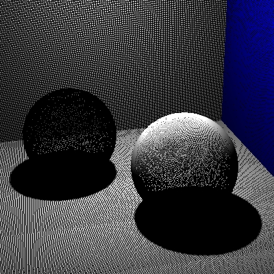
Here are two versions of the rendered image showing color bleeding:
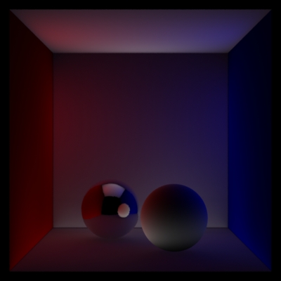 |
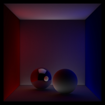 |
The shadows under the sphere are much darker in the image to the right due to "sortbleeding" being 1.
This example only shows the indirect illumination. If the shader also computes the direct illumination, a full global illumination image can be rendered.
If the indirectdiffuse() function is passed a parameter called "occlusion" it will also compute point-based approximate ambient occlusion and assign it to that parameter. If the indirectdiffuse() function is passed a parameter called "environmentdir" it will compute an environment direction (average unoccluded direction, also known as "bent normal").
The computation of color bleeding can be combined with environment map illumination -- just as for occlusion. Simply pass an "environmentmap" parameter to the indirectdiffuse() function.
It is important to note that there is very little run-time increase from computing occlusion to computing color bleeding. This is in contrast to ray tracing, where the cost of evaluating shaders at the ray hit points is often considerable.
Here is an example of point-based color bleeding in a more complex scene:
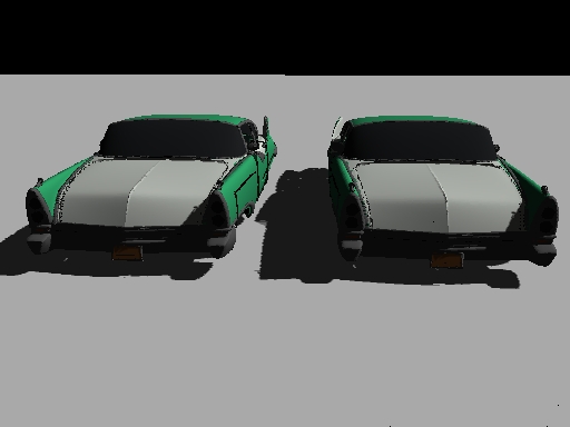 |
 |
Generating this radiosity point cloud takes about three minutes on a standard PC, and computing (and rendering) the point-based color bleeding takes around 9 minutes. Notice the strong green color bleeding from the cars, and the gray color bleeding from the ground onto the cars.
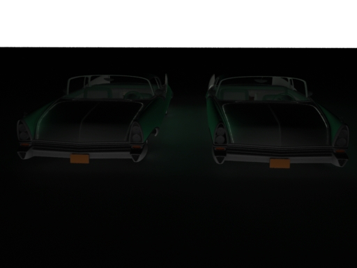
Illumination from area light sources can be computed as a special case of color bleeding.
The first step is to bake a point cloud with colored points from the light source objects, and black points from the shadow caster objects. The light sources and shadow casters can be any type of geometry, which makes this approach very flexible -- the geometry can even be displacement-mapped. The light source intensity can be constant or computed procedurally or using a texture.
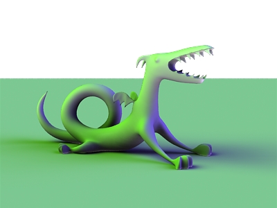
The following example shows three area light sources: a teapot, a sphere, and a dragon. The area lights illuminate a scene with three objects: a dragon, a sphere, and a ground plane.
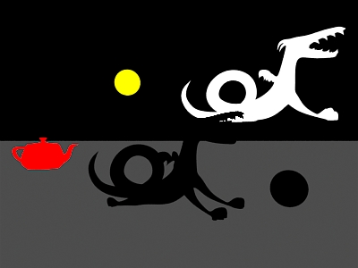 |
The result of this rendering is a point cloud containing very bright points from the light sources and black points from the shadow-casting objects. (For this scene, no points were baked from the ground plane since it is neither supposed to emit light nor cast shadows.)
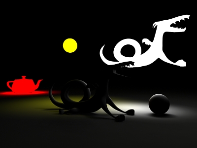
For this step, the same shader (pointbasedcolorbleeding) as above is used. it is important to set (keep) the "clamp" and "sortbleeding" parameters to 1. The image below shows color bleeding computed from the area light source point cloud:
 |
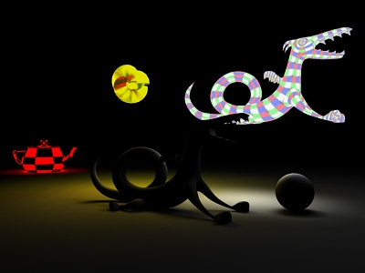
Below is another variation of this scene. Here the teapot light source has a procedural checkerboard texture, the sphere light source is displacement-mapped and texture-mapped, and the dragon light source is texture-mapped as well. (In this image, the light source objects are rendered dimmer than the colors used for baking their emission -- this is to avoid over-saturation that makes the textures hard to see.)
 |
Instead of rendering the occlusion and/or color bleeding, it can be useful to compute the data as a point cloud. This makes later reuse simple, and also makes it possible to generate a brick map (which has better caching properties than point clouds) of the data.
ptfilter -filter occlusion [options] areafiles occlusionfileThe last filename is the name of the resulting occlusion point cloud file; all preceeding filenames are the names of the (source) area point cloud files. For example:
ptfilter -filter occlusion -maxsolidangle 0.05 foo_areas.ptc foo_occl.ptc
This generates a point cloud with occlusion data. Optional parameters for ptfilter in occlusion mode are:
The computed occlusion point cloud for the simple scene looks like this:
 |
 |
The point cloud can now be used to generate a brick map of the occlusion values, if desired:
brickmake simple_occl.ptc simple_occl.bkm
As mentioned above, set the optional -envdirs parameter to 1 if the environment directions should be computed in addition to the occlusion. For example:
ptfilter -filter occlusion -maxsolidangle 0.05 -envdirs 1 foo_areas.ptc foo_occl.ptc
Here are the computed environment directions in the resulting point cloud:
 |
Ptfilter cannot currenly compute environment illumination.
For added flexibility, it is also possible to separately specify the positions where occlusion should be computed. The positions are given by points in a separate set of point cloud files. The syntax is as follows:
ptfilter -filter occlusion [options] -sources filenames -positions filenames -output filenameFor example:
ptfilter -filter occlusion -maxsolidangle 0.1 -sources foo_areas.ptc -positions foo_pos.ptc -output foo_occl.ptcIn this example there is only one file with areas and one file with positions; but each set of points can be specified by several point cloud files. If no position files are given, the point positions in the area point clouds are used.
Similar to the point-based occlusion computation, ptfilter can also compute color bleeding. This is done as follows:
ptfilter -filter colorbleeding -maxsolidangle 0.05 -sides front foo_radio.ptc foo_bleed.ptc
Use the command-line parameter -clamp if the computed color bleeding is too bright. The other command-line parameters are the same as for the occlusion filter.
Here are two different views of the color bleeding point cloud for the Cornell box scene:
 |
 |
Just as for occlusion computations, there can be a separate set of point clouds specifying where to compute the color bleeding.
Ptfilter can also compute multiple bounces of color bleeding. To do this, the original point cloud file must contain Cs data in addition to the area and radiosity data. Specify the desired number of bounces with the command-line parameter -bounces i. (The default value is 1.)
The data in the computed point cloud file are called "_occlusion" and "_indirectdiffuse" and optionally "_environmentdir".
Ptfilter can also compute soft illumination and shadows from area light sources. Simply bake a point cloud with brightly colored points at the area lights and black points at the shadow casters. Then run ptfilter -filter colorbleeding as in the previous section. Remember to set -clamp 1 and -sortbleeding 1 for best results.
The current implementation gives discontinuous, aliased results if "falloff" is set to 0 and "maxdist" is short (the default is 1e15). With short "maxdist" values, please use falloff 1 or 2.
If the computed occlusion or color bleeding is incorrect in a region of the scene, a good debugging method is to inspect the (area or radiosity) point cloud in that region using ptfilter in the disk or facet display mode. Is the disk representation of the surface a reasonable approximation of the original surface? If not, the shading rate for baking that object may need to be reduced in order to generate more, smaller disks that represent the surface better. If the area/radiosity point cloud is not a decent approximation of the surfaces, the point-based method cannot compute good results.
Some scenes are simply too complex to be ray traced — storing all the geometry uses more memory than what is available on the computer. For such scenes, point-based occlusion may be the only viable way to compute occlusion. As mentioned earlier, the area point clouds can be sparser than the accuracy of the final rendering, so even ridiculously complex scenes can be handled.
The advantage of using ptfilter rather than the occlusion() function to compute the point-based approximate ambient occlusion is most evident if the original area point cloud is very big (since occlusion() reads in the entire point cloud). If ptfilter has computed the occlusion, and the occlusion point cloud has been used to generate an occlusion brick map, we can just read bricks on demand. The disadvantage is that the occlusion point clouds have to be generated at quite high resolution, and the ptfilter'ing and brickmake'ing takes time.
Another use of point-based occlusion is in a workflow that computes occlusion for each frame. Each frame is first rendered coarsely to generate a rather sparse area point cloud. Then the frame is rendered with occlusion using the occlusion() function (with "pointbased" 1) at final resolution. The resulting image can be used as a 2D occlusion layer for compositing, and the point cloud can be deleted. Note that this workflow does not involve any point clouds or brick maps that have to be kept in the file system; the only result that is kept for later compositing is the full-frame occlusion-layer image.
| Pixar
Animation Studios
|