Prev |
Next
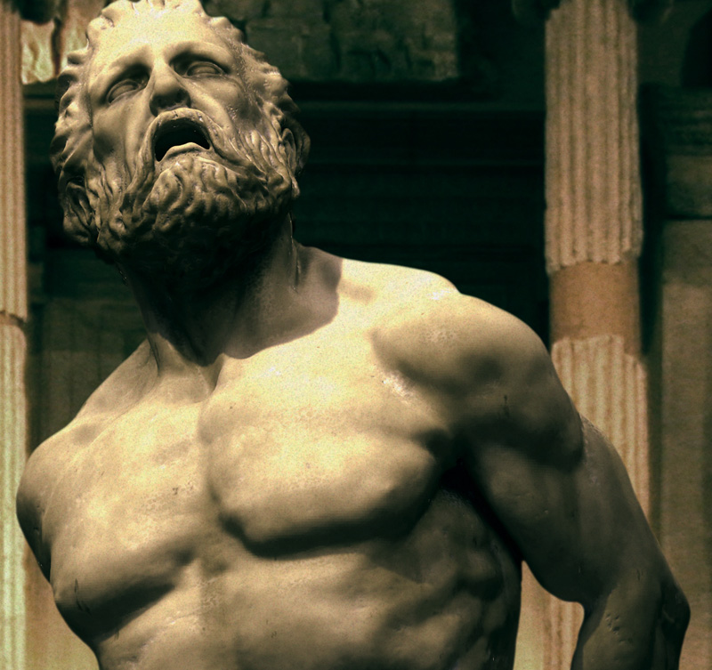
Prometheus — Rendering a
Greek God
|
The Prometheus tutorial was created by guest author, Scott
Eaton, of Escape Studios in London.
In the Prometheus tutorial, we will use RenderMan for Maya to shade, light and integrate a
3D model into a background plate from the British Museum. During the process, we will explore many of the advanced features that
RenderMan for Maya offers including: micropolygon displacements, subsurface scattering, ambient occlusion, brickmaps,
and secondary outputs. The tutorial will be broken into three
parts:
First, we will develop of a marble shader that approximates the main surface characteristics our reference images. It will need to show small divots from the wear of time on the surface of the marble, discoloration from oxidation, and changes in specularity from polished areas to rough, unfinished areas. And, of course, no marble shader would be complete without subsurface scattering.
As the shading network builds up, refer to the Maya materials in the scene files. Each important node will have notes on it to explain its function in the shading network.
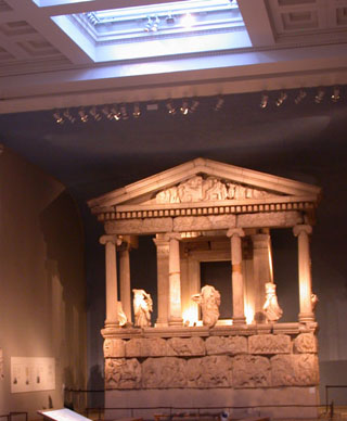
Second, we will analyze and match the lighting setup in the British Museum. Without the benefit of an HDRI probe to light from directly, we will have to dissect the lighting from reference photos and an analysis of how sculptures are lit in the British Museum.
Third, we will render out a number of secondary outputs (diffuse, specular, occlusion, etc) with RenderMan for Maya, and use
these secondary outputs to build up a composite over a background plate from the museum. This step is where the magic and flexibility of secondary outputs pays off as we layer and correct each output to match the museum plate.
|
|
|
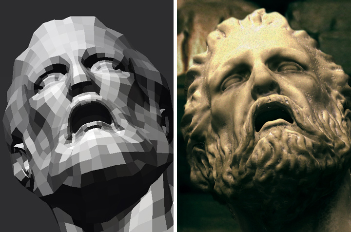
Before and After - In this tutorial we'll add
complexity to a simple model using displacements,
occlusion, subsurface scattering, and secondary outputs
|
This is an advanced tutorial combining a number of different workflows, and
because of that, this tutorial requires a good understanding of RenderMan for
Maya. You may need to review certain techniques elsewhere. A key strategy of
this tutorial is the use of Secondary Outputs, which will allow us to use 2D
compositing to finalize our lighting. At the end of the tutorial, the final result should look something like this:
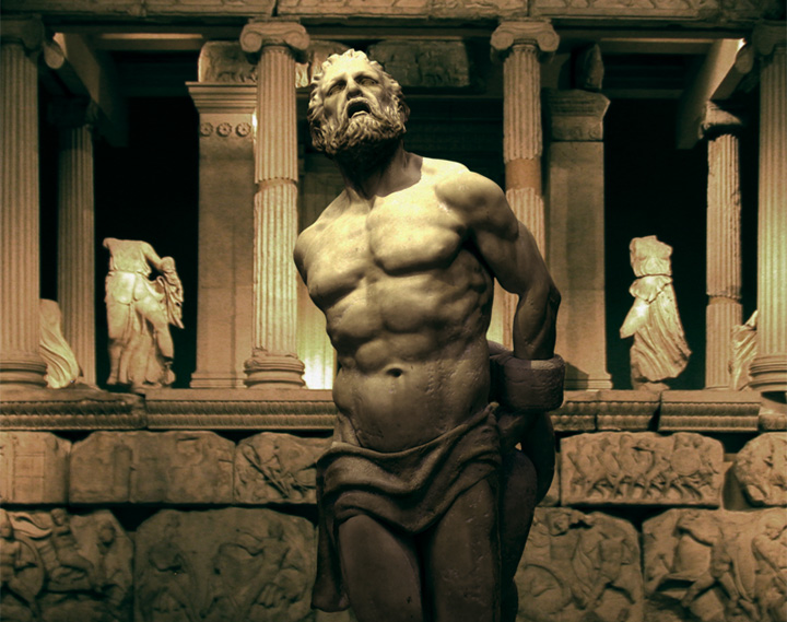
The end result,
the 3D model of Prometheus composited over the background image.
|
1 — ANALYZING
REFERENCE MATERIAL |
Before we get started, open Maya and make sure that RenderMan for Maya is properly set
up.
Weathered marble shader reference
1. The surface we are trying to mimic is aged, weathered marble. In our reference
image above, we can see that marble is not simply a 3D marble texture mapped onto a Blinn material. The surface is actually a layered combination of cloudy-grey base texture, yellowish surface discoloration from environmental wear, black specs from mineral contamination, faint rain streaks, and whitish marble dust build-up in the deep cavities.
Creating a convincing marble will be a challenge.
2. The lighting in the gallery is made up of both direct and indirect light sources.
In our reference photo above we can attribute a large amount of non-directional diffuse light to the skylight above the gallery. In addition, each sculpture is individually lit with warm,
colored spot lights located near the ceiling.
3. Open the Maya tutorial scene, Stage1.mb, to get started on the tutorial. (Where are the tutorial files?) The initial scene
contains a simple light setup and the three parts of our statue: Prometheus,
cloth, and chains. Our first step is to add comlexity to this
model using displacement maps.
|
2 — SHADING: SUBDIVISION AND
DISPLACEMENT |
4. We will begin by adding displacement maps to the 3D model which will add the intricacies of
a carved marble
statue to our lightweight 3D model. Luckily for us, we already
have displacement maps for this purpose, originally created using ZBrush. Because it is capable
of producing high quality displacement maps, ZBrush is a useful tool for use
with RenderMan because RenderMan is capable of rendering these displacement maps
extremely efficiently.

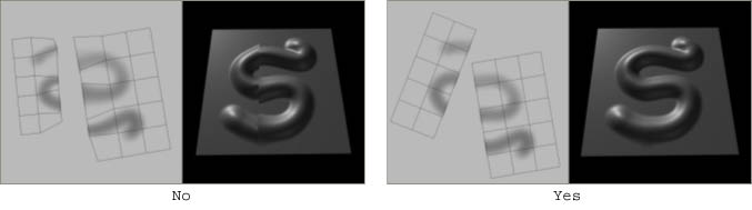
Watch UV Seams: When rendering displacement maps it is important to
create equal UV seams, otherwise artifacts may appear in the displacement along
the UV seams. In the images below, the image on the left has unequal seams,
while the image on the right has equal seams.
For the highest quality displacements, we'll want to render the model as a subdivision surface. In RFM, this is as easy as adding a single attribute to the shape node. Select
each piece of the statue, one piece at a time, and in the attribute editor select:
Attributes-> RenderMan-> Add Subdivision Scheme. Do a test render
to confirm that you have a perfectly smooth subdivision surface.
Three Blinn materials with displacements are added to the
three parts of the statue
5. Connect three standard Blinn materials to each of the three pieces of the
statue, and assign a file texture as a displacement map, as shown above. Get the 32bit displacement maps for each model from the source images
directory, sourceimages-> prometheus_tutorial-> [image folders]. In each file
node set the
Alpha Gain to 20, Alpha Offset to -10. This centers the displacement on 0. A final task: on
the file node, turn Filter Type to off. This stops filtering on the displacement map, which can reveal seams.
Displacement mapping: RenderMan for Maya brings RenderMan's extremely fast and accurate displacement mapping to Maya users. Getting used to having all this power takes time and a shift in thinking about geometric detail. Because RenderMan renders displacement mapping as quickly as bump mapping (nearly), there is no reason not to use it extensively in your scenes where geometric detail is required. Think, for example, tire treads on a large truck, a stone wall, etc. All can be represented in your scene with lightweight models but displaced at render time for maximum detail. Experiment by mapping a few procedural textures to a displacement node.
Displacement Attributes are added to the shader and
Displacement Bound is set to "20"
6. It is important to tell RenderMan how much you ever intend to displace your surface. This helps the renderer to efficiently process the geometry for rendering. Select
each of your displacement nodes and
go to Attributes-> Renderman-> Add Displacement Attrs, as shown
above. To estimate your displacement bound, roughly use your alpha gain from your displacement map
node, in this case "20".
"Trace Displacements" are enabled
7. We must also tell RenderMan that we want to use the displacement mapped version of this object for any ray tracing that we are going to do (occlusion, blurred reflections, etc). To do this we must add another RenderMan attribute to the shape node of our models. Individually select each shape
node, of the three parts of the statue, and go to
Attributes->RenderMan->Manage Attributes, then select and add Trace
Displacements.
Quality Control: A single parameter, Shading Rate, controls the quality of shading and displacement sampling in Renderman for Maya. The control is located in the
Render Settings-> Quality tab. The control is simple but powerful. The value is expressed in pixels and equates to the pixel space between shading samples (in screen space) at
render time. Therefore, the lower the number, the higher the quality. A value of one, for example, samples textures and procedural networks once for every pixel in the image; similarly a value of five samples every fifth pixel, and is quicker, but lower quality. Consider raising the shading rate to 5-10 to speed your preview renders, but drop it back down to
1.0 or 0.5 for final renders.
|
3 — SHADING: DIFFUSE, SPECULAR,
AND SUBSURFACE SCATTERING |
The network for the marble shader in the Maya file,
Stage2.mb
8. Next, we can build up the patterns from our reference with a combination of procedural textures, high-level control maps, and texture maps.
Now we'll take a shortcut and open
Stage2.mb and investigate how the marble shader is constructed.
Notice that the diffuse, specular, and bump components are built up using layers, many of which are shared between shading components. We will
use this network as the starting point for adding
RenderMan specific features to our materials.
Shading in Layers: It is good practice to break your shading up into modular layers. If you are building up a diffuse color (either procedurally or by painting maps), build it in components, starting from the largest "low frequency" patterns and work your way to smallest "high frequency" details. By separating these patterns into layers, it makes it easy to change or modify any one component independently. You will also find that some of these patterns will individually effect the specularity, reflectivity, or bump of the material and can be easily reused there. You will see extensive use of Layered Texture nodes in this shading network provided.
Add subsurface scattering attributes to the Blinn materials
and adjust as shown
9. Next add RenderMan subsurface scattering attributes to our three Blinn shaders. Select
each Blinn material and go to the attribute editor and add
RenderMan Attributes-> Subsurface Scattering. This adds a collection of extra attributes to the shader as well as an additional render pass for creating the SSS brickmap (which also shows up in the
Render Settings-> Passes tab).
Set the three Blinn's to share the same Brickmap Pass
10. For the SSS pass we want to include all three pieces of the statue into one pass
in order to share the brickmap between the three Blinn shaders. In each Blinn, right click over the
Scattering Map field and select the first rmanSSMakeBrickmapPass (delete
the other SSS passes from the
RenderSettings-> Passes tab). Now all three pieces of geometry will
be written to and read from one brickmap.
Configure the camera and set for the SSS pass
11. In Render Settings-> Passes, select the rmanSSRenderPass.
To pick the baking camera, right-click in the Camera field and select
bakingCameraShape, which has already been set up in the scene. To tell the pass which objects to render in the SSS pass, right-click in the
Sets field and choose
statueSet. (Note: for best SSS baking results, either enable raytraced shadows on lights or have shadow maps being reused, otherwise your SSS pass will not self shadow).
Now you're ready to render the effect. Remember that once the SSS effect is
rendered, the SSS brickmap can be reused. Since this statue is stationary and
the lights are fixed, we'll be able to reuse the SSS brickmap over and over.
Next render the effect then switch the Caching Behavior of the SSS
brickpass from Compute to Reuse, as shown in the following tip.
Reusing Brickmaps: Bake early, bake often. RenderMan uses an elegant baking system to capture computationally expensive effects into
3D caches called brickmaps. It is important understand that baking is done as a separate render pass, and
to get best results you should specify a reference camera in the Render Pass
settings. By changing the Caching Behavior of the pass you are able
to explicitly control the reuse of the SSS brickmap.
Caching Behavior can be set to
Compute, Reuse, or Disable
Add shadows to the spotlights
12. With the shaders finished, we can now focus on lighting. The
scene has two main lighting elements,
the spot lights and the sky light. To start, we'll tackle the spot lights.
There are four yellowish spotlights that light the sculpture from above. On each
of these spot lights, enable depth map shadows.
The shadow pass
13. Next we'll render the scene once to generate all our shadow maps, and then
we'll set our spot lights to reuse the shadow maps, so that they are not
recomputed every time we render. To reuse shadows, change the Disk Based Dmaps
setting on each spot light from Overwrite existing Dmaps(s) to Reuse existing
Dmaps(s).
Map Reuse: RenderMan has a long history of reusing pre-computed maps to save on render time for large productions. Each time you create a new pass that needs to compute a map (be it a shadow map, a reference map, or 3d brick map) you get a
Phase option to create a disk cache in two ways: once per job and
every frame. For stationary, non deforming geometry (as we have in this tutorial)
once per job is the option you want to select. For animation sequences where there is motion that will change the map, use
every frame and you will get a cached map for each frame of the animation.
14. To give us control over the shadow filtering and samples once we have a shadow mapped baked, we need to add additional custom attributes to our light shape node. Select the light and go to
Attributes->Renderman-> Shadow Attributes. This gives us access to the shadow filtering and shadow sampling attributes to blur the edges of our shadow maps as necessary.
Now the spot lights are properly set up.
15. Next we'll approximate the skylight in the British Museum.
To achieve this, we will combine two effects: an area light for specular
highlights and a custom occlusion pass (see next step) for soft shadowing. The area light will be used only to cast accurate specular reflections while the custom occlusion pass will allow us to bake expensive soft shadow calculations. Find the
areaSkylight in the scene, unhide it, and enable Emit Specular only.
16. Additionally, in the museum there is light reflected from the floor which is
cast from the overhead skylight. To create that effect, unhide the ambient light in
the scene ( we will later use the light to attenuate our ambient occlusion
pass). Set your intensity low and tune
Ambient Shade to 0.2 to give a little direction to our light, to simulate reflection from the ground. The amount of ambient can be tuned later in compositing.
|
5 — OCCLUSION AND SECONDARY
OUTPUTS |
Set up your environment light as shown
17. To create realistic shadowing, we'll add the global illumination effect,
ambient occlusion. To enable global illumination effects, (ambient occlusion
in this case) we must create a RenderMan environment light from the
RenderSettings-> Features tab. Enable RayTracing and create an
Environment Light. The environment light is where we access all our setting for occlusion. Tune the settings as shown, hide your other lights, and render. You should get a classic occlusion result.
(If not, make sure your Max Dist is set to "50".) Tune your settings until you are happy.
18. To save recalculating this expensive ray tracing effect every frame, we are going to bake the calculation into a
brickmap. First, create a new
MakeGlobalDiffuse3d pass in the Bake field of the Environment Light. This will create a new pass in the
Render Settings -> Passes tab where you can tune the Caching Behavior
and Phase for the pass. We will use compute and once per
job, as shown above.
Configure the RenderDiffuse3d pass as shown
19. The other tab created with the new MakeDiffuse3d pass is the RenderDiffuse3d pass, found
beside the former tab in the Render Settings. Similar to the SSS setup, this tab is where we setup a camera for final baking. Specify the same
bakingCameraShape, and then disable Cull Backfacing and Cull
Hidden. Add the RenderMan attribute Dice Rasterorient and disable it.
Render to bake, then set Caching Behavior in the MakeGlobalDiffuse3d
tab from Compute to Reuse.
Quality vs. Speed: The environment light has a number of parameters for tuning the type, quality and
speed of the global illumination effects. MaxVariation controls the amount of interpolation between
pixels and is analogous to Shading Rate: try setting this to 1 (or less) for
production quality and 10 (or more) for preview rendering.
20. Now we will simulate the illumination of the skylight. We will fake an area light using
ambient occlusion, because ambient occlusion makes it easy to bake this data
into a brickmap (unlike an actual area light). Hide your first environment light, and unhide the
occlusionBlocker mesh in the geometry group. This missing face at the top will act as the skylight letting the occlusion pass see white. Next create new environment light
(a second environment light) from the
Render Settings-> Features tab by right-clicking on the Environment
Light field.
21. We will make this Environment Light act like an area light by setting the Max Distance attribute to a value larger than the maximum dimension of our blocking geometry. Here a value of 10,000 is used. The other settings are the same as the last Environment Light.
22. Use similar bake settings for this pass. Remember to turn off Cull Backfacing,
Cull Hidden and Dice Rasterorient and specify the bakingCameraShape. Now render the scene to bake the occlusion brickmap. You should see this brickmap file, along with the other brickmaps, ptc files, and shadow maps is your /renderman/$scene/data folder in your current project (these default directories can be changed in the
Render Settings-> Advanced tab).
Add secondary outputs to the Final Pass
23. Now we will create the secondary outputs for compositing the final image.
First unhide all the lights, except the fist environment light which should
remain hidden. To prepare output passes we go to Render Settings-> Passes
tab. Here we add the following secondary outputs to our Final Defaults pass:
diffuse (DiffuseDirect), occlusion (OcclusionDirect), ambient (Ambientlight),
specular (SpecularDirect), subsurface scattering (Subsurface),
& surface color (DiffuseColor). Add these passes by clicking on the
black arrow next to Pass and selecting Final Defaults. Next click
on the black arrow next to the Output field and select the outputs one at
a time. Set all
outputs to format Tiff16. Render once in batch mode and look at your
secondary outputs, which will appear in the Maya project directory, renderman->
prometheus-> images. To get our original "close occlusion" pass, unhide our first envLight and hide the
second "skylight" envLight. Render with only occlusion as a secondary
output, and to do that you must delete the other secondary outputs by selecting
and deleting them from the pull-down menu. To prevent the first occlusion pass
from being overwritten, change its name to occlusion_arealight.tif.
Secondary Outputs: Rendering your scene in separate passes give you maximum flexibility in compositing and greatly reduces the amount of time you need to spend tuning your renders in
3D. RenderMan efficiently generates all the passes you need to rebuild a final render in compositing. Passes are known as secondary outputs in RenderMan, and the renderer is very efficient about
outputting these component parts from a single render (any number of outputs are
created at one time). Once you start using secondary outputs in compositing and you won't go back. When you break your output down into its component parts: diffuse, reflectivity, occlusion, shadow, etc., you have greater flexibility in color correcting individual layers to more precisely match background plates in hue, saturation, expose, etc.
Layer the secondary outputs with diffuse on bottom
24. The power of rendering with secondary outputs is that it gives you incredible control over tuning the look of your plate in
2D. For this example, we will use Photoshop to demonstrate the basic steps used to composite our secondary
outputs, although in a studio compositing might be performed with a dedicated
compositing program. For user's of RenderMan Studio, the image tool
"it" may be used to perform compositing (see below). Now using
Photoshop, open all your secondary outputs and layer them in one image as shown
above.
Adjusting lighting in compositing can be much faster than rerendering
25. Now we need to set the blending modes between layers. Diffuse is the lowest layer and above it screen on the
ambient channel. Next multiply by the close-occlusion layer. Then either multiply by the area light occlusion to take light out of the image, or screen to add light. Then overlay the
surfacecolor pass. Finally screen both the subsurface and specular passes. Use level adjustments to tune the image.
The final composite
26. Finally we color correct our plates to match the background. The main challenge of color correction is finding the correct transition from light to shadow and then matching the color temperature in the highs, mids, and shadows. Here the background plate is very warm red-orange in the mids and highs, while the shadows have more cyan. The final match was done using a combination of color balance for the temperature and levels for transitions.
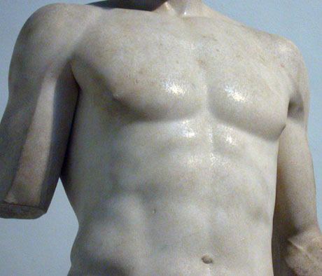
Closeup detail
About the Author: Scott Eaton is currently Creative Technical Director at
Escape Studios in London, where he divides his time between production and lecturing. His client list includes Sony, Microsoft Game Studios, The Mill, Double Negative, and many other leading production houses and games studios. Scott received his master's degree from the MIT Media Lab and subsequently studied traditional fine art at the Florence Academy of Art, Italy.
Prev |
Next
|
Pixar Animation Studios
Copyright©
Pixar. All rights reserved.
Pixar® and RenderMan® are registered trademarks of Pixar.
All other trademarks are the properties of their respective holders. |