Translucency and Subsurface Scattering
October 2002 (Revised December 2005)
![]()
Translucency and Subsurface ScatteringOctober 2002 (Revised December 2005) |
|
|
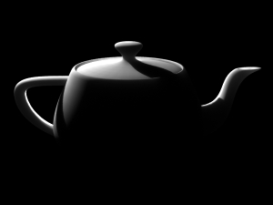
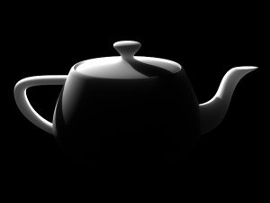
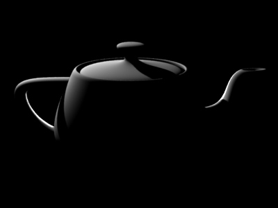
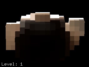
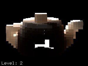
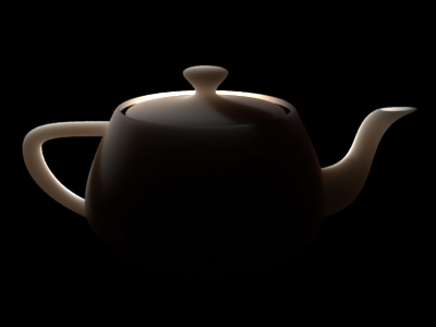
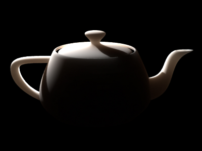
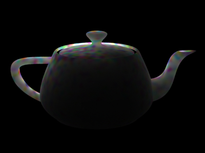
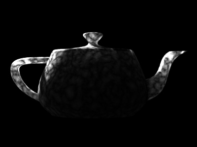
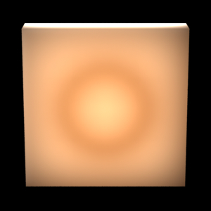
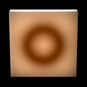
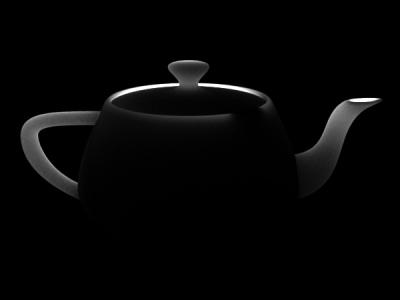
This application note describes how to simulate various aspects of subsurface scattering using Pixar's RenderMan (PRMan). The images below illustrate a simple example of subsurface scattering rendered with PRMan. The scene consists of a teapot made of a uniform, diffuse material. The teapot is illuminated by two spherical area lights (casting ray traced shadows), one very bright light behind the teapot and another light to the upper left of the teapot. There is no subsurface scattering in the first image, so the parts of the teapot that are not directly illuminated are completely black. In the second image, the material of the teapot has subsurface scattering with a relatively short mean path length, so the light can penetrate thin parts, such as the handle, knob, and spout, but very little light makes it through the teapot body. In the third image, the mean path length is longer, so more light can penetrate the material and even the teapot body is brighter.

|
|
|
In Section 2, we describe an efficient two-pass method to compute multiple scattering in a participating medium. In Section 3, we briefly discuss how to compute single scattering. In Section 4, we describe how to compute light transmission (without scattering) through a medium. Depending on the material parameters and the desired effects, one or several of these rendering methods can be chosen. For materials — such as human skin — that have high albedo, multiple scattering is much stronger than single scattering. In such cases, single scattering can be omitted.
    surface
    bake_radiance_t(string filename = "", displaychannels = ""; color Kdt = 1)
    {
        color irrad, rad_t;
        normal Nn = normalize(N);
        float a = area(P, "dicing"); // micropolygon area

        /* Compute direct illumination (ambient and diffuse) */
        irrad = ambient() + diffuse(Nn);

        /* Compute the radiance diffusely transmitted through the surface.
           Kdt is the surface color (could use a texture for e.g. freckles) */
        rad_t = Kdt * irrad;

        /* Store in point cloud file */
        bake3d(filename, displaychannels, P, Nn, "interpolate", 1,
               "_area", a, "_radiance_t", rad_t);

        Ci = rad_t * Cs * Os;
        Oi = Os;
    }
We bake out the area at each point. The area is needed for the subsurface scattering simulation. NOTE: It is important for the area() function to have "dicing" as its optional second parameter. This ensures that the shader gets the actual micropolygon areas instead of a smoothed version that is usually used for shading. (Alternatively, the shader can be compiled with the '-nosd' option to get the same (non-smoothed) micropolygon areas from the area() function.) Without this, the areas will be, in general, too large, resulting in subsurface scattering simulation results that are too bright.
The optional parameter "interpolate" makes bake3d() write out a point for each micropolygon center instead of one point for each shading point. This ensures that there are no duplicate points along shading grid edges.
To ensure that all shading points are shaded, we set the attributes "cull" "hidden" and "cull" "backfacing" to 0 in the rib file. We also set the attribute "dice" "rasterorient" to 0 to ensure an even distribution of shading points over the surface of the object. The rib file for baking the diffusely transmitted direct illumination on a teapot looks like this:
    FrameBegin 1

      Format 400 300 1
      ShadingInterpolation "smooth"
      PixelSamples 4 4
      Display "teapot_bake_rad_t.rib" "it" "rgba"   # render image to 'it'
      Projection "perspective" "fov" 18
      Translate 0 0 170
      Rotate -15  1 0 0
      DisplayChannel "float _area"
      DisplayChannel "color _radiance_t"

      WorldBegin

        Attribute "visibility" "int diffuse" 1   # make objects visible for raytracing
        Attribute "visibility" "int specular" 1
        Attribute "visibility" "int transmission" 1
        Attribute "shade" "string transmissionhitmode" "primitive"
        Attribute "trace" "bias" 0.01
        Attribute "cull" "hidden" 0   # don't cull hidden surfaces
        Attribute "cull" "backfacing" 0   # don't cull backfacing surfaces
        Attribute "dice" "rasterorient" 0 # turn viewdependent gridding off

        # Light sources (with ray traced shadows)
        LightSource "pointlight_rts" 1 "from" [-60 60 60] "intensity" 10000 "samples" 4
        LightSource "pointlight_rts" 2 "from" [0 0 100] "intensity" 75000 "samples" 4

        # Teapot
        AttributeBegin
          Surface "bake_radiance_t" "filename" "direct_rad_t.ptc"
                                    "displaychannels" "_area,_radiance_t"
          Translate -2 -14 0
          Rotate -90  1 0 0
          Scale 10 10 10   # convert units from cm to mm
          Sides 1
          Geometry "teapot"
        AttributeEnd

      WorldEnd
    FrameEnd
The rendered image looks like this:
|
|
|
The point density is determined by the image resolution and the shading rate. If the points are too far apart, the final image will have low frequency artifacts. As a rule of thumb, the shading points should be spaced no more apart than the mean free path length lu (see the following).
In this example, the illumination is direct illumination from two point lights. It could just as well be high dynamic range illumination from an environment map or global illumination taking indirect illumination of the teapot into account.
The volume diffusion computation is done using a stand-alone program called ptfilter. The diffusion approximation follows the method described in [Jensen01], [Jensen02], and [Hery03], and uses the same efficient algorithm as was used for e.g. Dobby in “Harry Potter and the Chamber of Secrets” and Davy Jones and his crew in “Pirates of the Caribbean 2”.
The subsurface scattering properties of the material can be specified in three equivalent ways:
ptfilter -ssdiffusion -material marble direct_rad_t.ptc ssdiffusion.ptcThe built-in materials are apple, chicken1, chicken2, ketchup, marble, potato, skimmilk, wholemilk, cream, skin1, skin2, and spectralon; the data values are from [Jensen01]. The data values assume that the scene units are mm; if this is not the case a unitlength parameter can be passed to ptfilter. For example, if the scene units are cm, use -unitlength 0.1.
ptfilter -ssdiffusion -scattering 2.19 2.62 3.00 -absorption 0.0021 0.0041 0.0071 -ior 1.5 direct_rad_t.ptc ssdiffusion.ptc
ptfilter -ssdiffusion -albedo 0.830 0.791 0.753 -diffusemeanfreepath 8.51 5.57 3.95 -ior 1.5 direct_rad_t.ptc ssdiffusion.ptc
|
The accuracy of the subsurface diffusion simulation can be determined by the ptfilter parameter "-maxsolidangle". This parameter determines which groups of points can be clustered together for efficiency. (It corresponds to the 'eps' parameter of [Jensen02], page 579.) This parameter is a time/quality knob: the smaller value of maxsolidangle, the more precise but slow the simulation is. Too large values result in low-frequency banding artifacts in the computed scattering values. The default value for maxsolidangle is 1.
TIP: If you'd like to know which values of albedo, diffuse mean free path length, and index of refraction are being used for the subsurface diffusion simulation, you can add '-progress 1' to the ptfilter command-line arguments. In addition, '-progress 2' will write out some of the computed subsurface scattering values.
Next, the point cloud file with subsurface diffusion colors needs to be converted to a brick map file so that the texture3d() shadeop can read it efficiently. This is done as follows:
brickmake -maxerror 0.002 ssdiffusion.ptc ssdiffusion.bkm
The top 3 levels of the resulting brick map, ssdiffusion.bkm, are shown below (visualized with the interactive brickviewer program):
|
|
|
    surface
    read_ssdiffusion(uniform string filename = ""; float Ka = 1, Kd = 1)
    {
        normal Nn = normalize(N);
        color direct = 0, ssdiffusion = 0;

        /* Compute direct illumination (ambient and diffuse) */
        direct = Ka*ambient() + Kd*diffuse(Nn);

        /* Look up subsurface scattering color */
        texture3d(filename, P, N, "_ssdiffusion", ssdiffusion);

        /* Set Ci and Oi */
        Ci = (direct + ssdiffusion) * Cs * Os;
        Oi = Os;
    }
The rib file looks like this (the light sources are only needed for the direct illumination):
    FrameBegin 1

      Format 600 450 1
      ShadingInterpolation "smooth"
      PixelSamples 4 4
      Display "teapot_read_ssdiffusion.rib" "it" "rgba"   # render image to 'it'
      Projection "perspective" "fov" 18
      Translate 0 0 170
      Rotate -15  1 0 0

      WorldBegin

        Attribute "visibility" "int diffuse" 1   # make objects visible for raytracing
        Attribute "visibility" "int specular" 1
        Attribute "visibility" "int transmission" 1
        Attribute "shade" "string transmissionhitmode" "primitive"
        Attribute "trace" "bias" 0.01

        # Light sources (with ray traced shadows)
        LightSource "pointlight_rts" 1 "from" [-60 60 60] "intensity" 10000 "samples" 4
        LightSource "pointlight_rts" 2 "from" [0 0 100] "intensity" 75000 "samples" 4

        # Teapot
        AttributeBegin
          Surface "read_ssdiffusion" "filename" "ssdiffusion.bkm"
          Translate -2 -14 0
          Rotate -90  1 0 0
          Scale 10 10 10   # convert units from cm to mm
          Sides 1
          Geometry "teapot"
        AttributeEnd

      WorldEnd
    FrameEnd
The subsurface scattering image looks like this (with and without direct
illumination):
|
|
If desired, the shader can of course multiply the subsurface color by a texture and also add specular highlights, etc.
The example above had a uniform albedo and a uniform diffuse mean free path length. It is simple to multiply the transmitted radiance by a varying diffuse color prior to baking it. For another effect, we can also specify varying albedos and diffuse mean free paths in the diffusion simulation. This requires that we bake the albedo and diffuse mean free paths in the point cloud file along with the transmitted radiance.
Shader example:
    surface
    bake_sss_params(string filename = "", displaychannels = ""; color Kdt = 1)
    {
        color irrad, rad_t;
        color albedo, dmfp = 10;
        normal Nn = normalize(N);
        point Pobj = transform("object", P);
        float a = area(P, "dicing"); // micropolygon area
        float freq = 5;

        /* Compute direct illumination (ambient and diffuse) */
        irrad = ambient() + diffuse(Nn);

        /* Compute the radiance diffusely transmitted through the surface.
           Kdt is the surface color (could use a texture for e.g. freckles) */
        rad_t = Kdt * irrad;

        albedo = noise(freq * Pobj);

        /* Store in point cloud file */
        bake3d(filename, displaychannels, P, Nn, "interpolate", 1,
               "_area", a, "_radiance_t", rad_t, "_albedo", albedo,
               "_diffusemeanfreepath", dmfp);

        Ci = rad_t * Cs * Os;
        Oi = Os;
    }
The rib file is very much as in the previous example, but with more DisplayChannels and the bake_sss_params surface shader:
    FrameBegin 1

      Format 400 300 1
      ShadingInterpolation "smooth"
      PixelSamples 4 4
      Display "teapot_bake_rad_t.rib" "it" "rgba"   # render image to 'it'
      Projection "perspective" "fov" 18
      Translate 0 0 170
      Rotate -15  1 0 0
      DisplayChannel "float _area"
      DisplayChannel "color _radiance_t"
      DisplayChannel "color _albedo"
      DisplayChannel "color _diffusemeanfreepath"

      WorldBegin

        Attribute "visibility" "int diffuse" 1   # make objects visible for raytracing
        Attribute "visibility" "int specular" 1
        Attribute "visibility" "int transmission" 1
        Attribute "shade" "string transmissionhitmode" "primitive"
        Attribute "trace" "bias" 0.01
        Attribute "cull" "hidden" 0   # don't cull hidden surfaces
        Attribute "cull" "backfacing" 0   # don't cull backfacing surfaces
        Attribute "dice" "rasterorient" 0 # turn viewdependent gridding off

        # Light sources (with ray traced shadows)
        LightSource "pointlight_rts" 1 "from" [-60 60 60] "intensity" 10000 "samples" 4
        LightSource "pointlight_rts" 2 "from" [0 0 100] "intensity" 75000 "samples" 4

        # Teapot
        AttributeBegin
          Surface "bake_sss_params" "filename" "direct_and_params.ptc"
              "displaychannels" "_area,_radiance_t,_albedo,_diffusemeanfreepath"
          Translate -2 -14 0
          Rotate -90  1 0 0
          Scale 10 10 10   # convert units from cm to mm
          Sides 1
          Geometry "teapot"
        AttributeEnd

      WorldEnd
    FrameEnd
Rendering this rib file produces the point cloud file direct_and_params.ptc. The diffusion simulation is done by calling ptfilter like this:
ptfilter -ssdiffusion -albedo fromfile -diffusemeanfreepath fromfile direct_and_params.ptc ssdiffusion.ptc
The resulting point cloud file, ssdiffusion.ptc, has a varying ssdiffusion color. The point cloud is converted to a brick map just as before:
brickmake -maxerror 0.002 ssdiffusion.ptc ssdiffusion.bkm
Rendering the brick map is done using the same rib file as in section 2.4. The resulting image (without direct illumination) looks like this:
|
Here are a couple of other images of subsurface scattering with varying albedo:
|
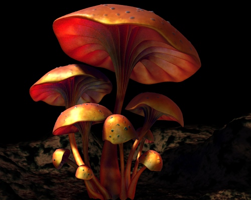
|
The diffusion approximation described above can not take blocking geometry such as bones into account. But sometimes we would like to fake the effect of less subsurface scattering in e.g. skin regions near a bone. This can be done by baking negative illumination values on the internal object; this negative subsurface scattering will make the desired regions darker.
The same shader as above, bake_radiance_t, is used to bake the illuminated surface colors. But in addition, we use a simple shader to bake constant (negative, in this case) colors on the blocker:
    surface
    bake_constant( uniform string filename = "", displaychannels = "" )
    {
        color surfcolor = Cs;
        normal Nn = normalize(N);
        float a = area(P, "dicing"); // micropolygon area

        bake3d(filename, displaychannels, P, Nn, "interpolate", 1,
               "_area", a, "_radiance_t", surfcolor);

        Ci = Cs * Os;
        Oi = Os;
    }
Here is a rib file for baking direct illumination on a thin box and negative color on a torus inside the box:
    FrameBegin 1

       Format 300 300 1
       ShadingInterpolation "smooth"
       PixelSamples 4 4
       Display "blocker_bake.rib" "it" "rgba"
       Projection "perspective" "fov" 15
       Translate 0 0 100
       Rotate -15  1 0 0

       DisplayChannel "float _area"
       DisplayChannel "color _radiance_t"

       WorldBegin

         Attribute "cull" "hidden" 0   # don't cull hidden surfaces
         Attribute "cull" "backfacing" 0   # don't cull backfacing surfaces
         Attribute "dice" "rasterorient" 0   # turn viewdependent gridding off

         # Light sources
         LightSource "pointlight" 1 "from" [-60 60 60] "intensity" 10000
         LightSource "pointlight" 2 "from" [0 0 100] "intensity" 75000

         # Thin box (with normals pointing out)
         AttributeBegin
           Surface "bake_radiance_t" "filename" "blocker_direct.ptc"
                                     "displaychannels" "_area,_radiance_t"
           Scale 10 10 2
           Polygon "P" [ -1 -1 -1  -1 -1 1  -1 1 1  -1 1 -1 ]   # left side
           Polygon "P" [ 1 1 -1  1 1 1  1 -1 1  1 -1 -1 ]       # right side
           Polygon "P" [ -1 1 -1  1 1 -1  1 -1 -1  -1 -1 -1 ]   # front side
           Polygon "P" [ -1 -1 1  1 -1 1  1 1 1  -1 1 1 ]       # back side
           Polygon "P" [ -1 -1 -1  1 -1 -1  1 -1 1  -1 -1 1 ]   # bottom
           Polygon "P" [ -1 1 1  1 1 1  1 1 -1  -1 1 -1 ]       # top
         AttributeEnd

         # Blocker: a torus with negative color
         AttributeBegin
           Surface "bake_constant" "filename" "blocker_direct.ptc"
                                   "displaychannels" "_area,_radiance_t"
           Color [-2 -2 -2]
           #Color [-5 -5 -5]
           Torus 5.0 0.5  0 360  360
         AttributeEnd

       WorldEnd
     FrameEnd
Rendering this rib file results in a rather uninteresting image and a more interesting point cloud file called "blocker_direct.ptc".
The next step is to do the subsurface scattering simulation. For this example we'll use the default material parameters. In order to avoid blocky artifacts it is necessary to specify a rather low maxsolidangle:
ptfilter -ssdiffusion -maxsolidangle 0.3 blocker_direct.ptc blocker_sss.ptc
Then a brick map is created from the subsurface scattering point cloud:
brickmake blocker_sss.ptc blocker_sss.bkm
To render the box with subsurface scattering we use the same shader, read_ssdiffusion, as in the previous sections. The rib file looks like this:
    FrameBegin 1

      Format 300 300 1
      ShadingInterpolation "smooth"
      PixelSamples 4 4
      Display "blocker_read.rib" "it" "rgba"
      Projection "perspective" "fov" 15
      Translate 0 0 100
      Rotate -15  1 0 0

      WorldBegin

        Surface "read_ssdiffusion" "filename" "blocker_sss.bkm"

        # Thin box (with normals pointing out)
        AttributeBegin
          Scale 10 10 2
          Polygon "P" [ -1 -1 -1  -1 -1 1  -1 1 1  -1 1 -1 ]   # left side
          Polygon "P" [ 1 1 -1  1 1 1  1 -1 1  1 -1 -1 ]       # right side
          Polygon "P" [ -1 1 -1  1 1 -1  1 -1 -1  -1 -1 -1 ]   # front side
          Polygon "P" [ -1 -1 1  1 -1 1  1 1 1  -1 1 1 ]       # back side
          Polygon "P" [ -1 -1 -1  1 -1 -1  1 -1 1  -1 -1 1 ]   # bottom
          Polygon "P" [ -1 1 1  1 1 1  1 1 -1  -1 1 -1 ]       # top
        AttributeEnd

      WorldEnd
    FrameEnd
Here are three images of the thin box with varying degrees of blocking:
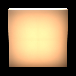
|
|
|
See [Hery03] for more discussion and examples of blocking geometry.
Single scattering is not important in materials such as skin. For other materials, where it is more important, it can be done in a shader using the trace() and transmission() functions.
Another effect that occurs in participating media is that some of the light from the surfaces travels straight through the medium without being scattered. Due to absorption, the amount of light that is transported this way falls off exponentially with the distance through the medium.
An object of frosted, colored glass is a good example of this type of light transport. The frosted surface of the glass scatters the light diffusely into the object. The internal part of the glass is clear and scatters very little light (but absorbs some of the light due to the coloring).
This effect can be computed by shooting rays with the gather construct. Basically, for each visible shading point, we want to shoot a collection of rays from that point into the object and look up the direct illumination at the surface points those rays hit.
So the shader needs to distinguish between whether it is running on a directly visible point or on a subsurface ray hit point. A ray label is used to communicate this information.
It is assumed that the surfaces have the correct orientation, i.e. that the normals are pointing out of the objects.
We first compute the direct illumination and store it just as in section 2.1.
brickmake -maxerror 0.002 direct_rad_t.ptc direct_rad_t.bkm
The brick map can be visualized using the brickviewer program.
A shader that renders light transmission with absorption (and direct illumination if so desired) with the help of a brick map of the direct illumination is listed below. The shader utilizes the convention that if the texture3d() call fails to find the requested value, it does not change the value of the 'rad_t' parameter. So in this shader, we can get away with not checking the return code of texture3d(): if it fails, rad_t will remain black.
    surface
    subsurf_noscatter(float Ka = 1, Kd = 1, Ks = 1, roughness = 0.1;
                      float Ksub = 1, extcoeff = 1, samples = 16;
                      string filename = "")
    {
        color rad_t = 0;
        normal Nn = normalize(N);
        vector Vn = -normalize(I);
        uniform string raylabel;

        rayinfo("label", raylabel);

        if (raylabel == "subsurface") { /* subsurface ray from inside object */

            /* Lookup precomputed irradiance (use black if none found) */
            texture3d(filename, P, Nn, "_radiance_t", rad_t);
            Ci = rad_t;

        } else { /* regular shading (from outside object) */

            color raycolor = 0, sum = 0, irrad;
            float dist = 0;

            /* Compute direct illumination (ambient, diffuse, specular) */
            Ci = (Ka*ambient() + Kd*diffuse(Nn)) * Cs
                 + Ks*specular(Nn,Vn,roughness);

            /* Add transmitted light */
            if (Ksub > 0) {
                gather("illuminance", P, -Nn, PI/2, samples,
                       "label", "subsurface",
                       "surface:Ci", raycolor, "ray:length", dist) {
                    sum += exp(-extcoeff*dist) * raycolor;
                }
                irrad = sum / samples;
                Ci += Ksub * irrad * Cs;
            }
        }

        Ci *= Os;
        Oi = Os;
    }
The image below shows the resulting light transmission through a teapot:
|
Rendering this image requires 6.3 million subsurface rays, so it is significantly slower than computing the diffusion approximation in section 2.
Q: Which method does ptfilter use to compute subsurface scattering?
A: We use the efficient hierarchical diffusion approximation by Jensen and co-authors -- see the references below.
Q: If I specify the material for the diffusiont simulation, how can I get to see the corresponding material parameters that are being used in the simulation?
A: Use the -progress 1 or -progress 2 flag for ptfilter -ssdiffusion. This prints out various information during the simulation calculation.
Q: I see banding in the subsurface scattering (diffusion) result produced by ptfilter. How can I get rid of the bands?
A: Decrease the maxsolidangle in ptfilter and/or increase the density of baked points (for example by decreasing the shadingrate or increasing the image resolution).
Q: The ptfilter diffusion computation is too slow. How can I speed it up?
A: Increase the maxsolidangle in ptfilter and/or decrease the number of baked points (for example by increasing shadingrate or decreasing image resolution).
Q: The brick map generated by brickmake is huge. How can I make it smaller?
A: Use maxerror values of 0.002, 0.004 or 0.01 or even higher in brickmake.
Q: What exactly is the maxsolidangle parameter of ptfilter's diffusion approximation?
A: Maxsolidangle is the parameter called epsilon on page 579 of [Jensen02].
Q: My subsurface scattering results has bright areas that roughly correspond to a shading grid. What's going on?
A: This is a problem that sometimes occurs if the point cloud has been generated in -p:2 mode: some grids get baked more that once. The workaround is to generate the point cloud without using -p:2. (It is, however, perfectly safe to generate the point cloud in multithreaded mode, for example -t:2.)
First of all, the illumination on the surface of the examples is purely direct illumination. It could just as well be high dynamic range illumination from an environment map or global illumination taking indirect illumination of the teapot into account.
Second, the 3D texture is only evaluated on the surfaces. In order to improve the accuracy of light extinction inside the object the 3D texture should be evaluated inside the object, too. This requires evaluation of the 3D texture at many positions along each subsurface ray.
More information about the methods we use for efficient simulation of subsurface scattering can be found in for example:
Information about PRMan's ray tracing functionality can be found in the application note “A Tour of Ray-Traced Shading in PRMan”. More information about point clouds and brick maps can be found in application note “Baking 3D Textures: Point Clouds and Brick Maps”.
The source code of our implementation of subsurface scattering is listed in section 8.3 of the application note “Baking 3D Textures: Point Clouds and Brick Maps”.
| Pixar
Animation Studios
|